High affinity interaction
When we have high affinity or strong interactions the kintic rate constants are not easily resolved due to the slow dissociation and by the fact that reaching equilibrium takes a long time.
Characteristics of a high affinity interactionA high affinity interaction is commonly determined by a low dissociation rate (<10-5 s-1) and a relative low equilibrium dissociation constant (<10-9 M). Although a sufficient fast association rate enhances the forming of the complex, the dissociation rate determines the time that the two molecules stay together in complex. Even when one of the free molecules is removed, the complex of a high affinity interaction stays intact for a long time.
Time to steady state
As a consequence of the slow dissociation rate, the time to steady state is also prolonged compared to a faster dissociation rate. This means that the association time must be long enough to generate some curvature in the measurement even if steady state is not reached. Lines without curvature cannot be fitted uniquely. Ideally, one of the curves should reach at least 80% of the steady state response within the association time.
The problem with sub-nanomolar affinities is that it can take days or even weeks to reach equilibrium. The time to steady state is, however, also dependent on the association rate and the analyte concentration as shown in the formula below. The Greek letter theta (Θ) stands for the percentage Req to be reached (e.g. 95% Req: Θ = 0.95).

From the formula also follows that a higher analyte concentration will lower the time to equilibrium. Every doubling in analyte concentration will decrease the time by approximately one third. However, concentrations higher than 30 times the KD are not recommended since they may suffer from non-Langmuirian behaviour which makes the analysis more difficult.
Affinity plot
The affinity plot shows the relation between the association (ka) and dissociation (kd) rate constants and the equilibrium dissociation constant (KD).
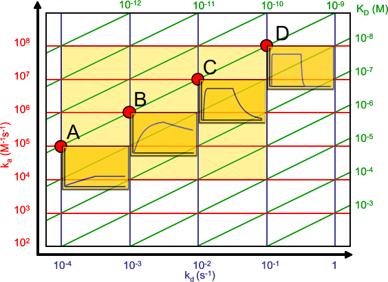
The association rate constants are on the y-axis in red. The dissociation rate constants are in blue on the x-axis. The intersection of the ka and kd gives an equilibrium dissociation constant in green. Hence the green lines connect the points with the same KD. The intermediate yellow box marks the range in which most of the association and dissociation rate constants can be expected. The four red dots show examples of the curves at the intersections (the analyte concentration is 1 nM = 1 x KD).
Although generally a high affinity is connected to slow dissociation rate, from the affinity plot it can be seen that this is not always the case. A high association rate (e.g. 106 M-1s-1) combined with an average dissociation rate (e.g. 10-3 s-1) can give a 1 nanomolar equilibrium dissociation constant. Therefore, some care must be taken comparing equilibrium dissociation constants alone.
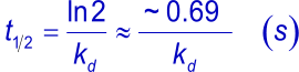
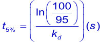
To measure strong interactions (slow dissociation rates) with SPR, long dissociation times are needed. Usually, dissociation is followed until enough data points are measured to ensure a valid fitting on the curves. To have a valid fitting, the decay in dissociation should be at least 5% of the initial response from the start of the dissociation. The time to reach the theoretical 5% decay can be calculated using the following formulas and are summarized in the tables below.
| kd | t½ | t½ | t½ |
|---|---|---|---|
| (s-1) | (s) | (min) | (h) |
| 1.10-1 | 7 | 0.1 | 0.0 |
| 1.10-2 | 69 | 1.2 | 0.0 |
| 1.10-3 | 693 | 11.6 | 0.2 |
| 1.10-4 | 6931 | 115.6 | 0.9 |
| 1.10-5 | 69315 | 1155.2 | 19.3 |
| 1.10-6 | 693147 | 11552.5 | 192.5 |
Examples of high affinity
One of the strongest interaction known is the binding between avidin and D-biotin (KD ≈ 10-15 M) or streptavidin and D-biotin (KD: 10-13 M) (1). One other interaction, which has often a high affinity binding, is the antibody–antigen interaction, although this is mainly due to the two binding sites of one IgG molecule. Interactions with a high affinity have a low equilibrium dissociation constant, generally in the range of 10-9 – 10-12 M.
In kinetics there seems to be a race for the best (lowest in this context) equilibrium dissociation constant (KD) there is. Interactions are compared by their equilibrium dissociation constant only and that is it. Similarly, often only the IC50 of a system is given while the full kinetics are not well established (2). In my opinion, reporting a single value for a kinetic interaction is obscuring all the other information present in the measurements between two or more components.
Using kinetic interaction methods such as surface plasmon resonance, bilayer interferometry or isothermal calorimetry (no ka or kd but stoichiometry and thermodynamic properties) the results contain more information than the equilibrium dissociation constant alone. In addition, these techniques make it possible to change the assay conditions (e.g. buffer composition, pH or temperature) to determine what their influence is on the kinetic constants.
When do you need high affinity?
Techniques like ELISA, purifications and drug-receptor binding benefit from high affinity interactions. Especially the low dissociation rate gives a high stability to the reaction which in turn provides a stable complex for a longer time. In addition, high affinity interactions can generally withstand more strict washing steps than low affinity interactions. In addition, a stable complex in a drug-receptor complex enhances the efficacy of the drug.
How to measure high affinity interactions with SPR?
As shown above, a slow dissociation rate needs a long dissociation time in order to have sufficient decay in the response. Longer dissociation times can suffer from drift and pump spikes when the flow pumps have to refill. A well equilibrated system is a prerequisite to measure long dissociation times. In addition, sufficient blank (buffer alone) runs are needed to perform the double referencing in order to compensate for active versus reference channel differences and to compensate for possible drift. In-line referencing is recommended but for double referencing blank runs are still necessary. In an experiment, only the highest analyte injections need to have a long dissociation time, making the process more efficient. This is referred to as the 'short and long' injection strategy (3),(4).
Mass transport can be a problem both in the association as in the dissociation phase. High density surfaces enhance mass-transport and the initial part of the binding curve will be linear. Since the association time is mostly limiting with high affinity interactions mass transport should be prevented. Low density surfaces with sufficient response (50 - 100 RU) are recommended. Similarly, the dissociation will benefit from low density surfaces as rebinding of the analyte is kept to a minimum. A higher flow rate can minimize rebinding. As an alternative to minimize rebinding the ligand can be injected during the dissociation phase but this reduces the dissociation time to the injection volume.
MCK and SCK
Both multi cycle (MCK) and single cycle kinetics (SCK) can be used to resolve slow dissociation rates. The multi cycle approach uses the short and long strategy with the long dissociation time during the highest analyte injections. Blank runs with the same long dissociation time serve as reference curves for the double referencing. The single cycle kinetics generally ends with a long dissociation.
Equilibrium analysis of interactions with a slow dissociation rate is difficult since the time to steady state becomes much longer. Generally, the injection volume is not sufficient to have such long injection times. A solution to overcome the injection volume problem is to add the analyte directly to the flow buffer and recirculate it until steady state is reached (5). Then the analyte concentration is increased and recirculated until a new steady state is reached. In this way several steady state points can be obtained. After the highest analyte concentration, the buffer is replaced by clean flow buffer and the dissociation is monitored until enough response is decayed.
Solution affinity
Solution affinity measures the equilibrium dissociation constant and the stoichiometry of the binding between two interactants in solution (6). Mixtures of protein and analyte are equilibrated outside the instrument and the concentration of the unbound analyte is determined with SPR under mass transport limitation. The advantage of solution affinity measurements is that the incubation between ligand/analyte (receptor/ligand) can be done outside the instrument for a very long time to reach true equilibrium. In addition, neither binding partner has to be labeled and only the protein to determine the free analyte has to be immobilized. One pre-requisite is that the ligand/protein surface only detects the free analyte and not the analyte-protein complex or the ligand/protein itself.
Instrument resolution
To be able to measure high affinity interactions, the instrument must be capable of doing this. In general this concerns the injection volumes, long and short-term noise, drift and the run time with flow buffer (data file size). Especially the drift during dissociation can be a problem since the dissociation rate is slow. Proper set-up of the instrument (buffer equilibration, reference channel(s)) and experimental design (enough decay during dissociation, double referencing) maximizes the measuring range.
| Instrument | ka (M-1s-1) | kd (s-1) | KD (M) |
|---|---|---|---|
| Biacore 2000 | 103 – 5.106 | 5.10-6 – 10-1 | 10-4 – 2.10-10 |
| Biacore 3000 | 103 – 107 | 5.10-6 – 10-1 | 10-4 – 2.10-10 |
| Biacore T200/S200 | Proteins: 103 – 3.109 | ||
| LMW molecules: 103 – 5.107 | 10-5 – 1 | 10-3 – 3.10-15 | |
| Biacore X100 | 103 – 107 | 1.10-5 – 10-1 | 10-4 – 1.10-10 |
| Biacore 8K | 103 – 3.109 | 10-6 – 0.5 | 5.10-4 – 3.10-15 |
| BioNavis 220A NAALI | 103 – 108 | 10-7 – 10-1 | 10-3 – 10-12 |
| ForteBio Pioneer | <108 | 1.10-6 – 10-1 | 10-3 – 10-12 |
| Nicoya OpenSPR | 103 – 107 | 10-5 – 10-1 | 10-3 – 10-12 |
| IBIS-MX96 | 5.102 – 5.106 | 2.10-6 – 5.10-2 | 10-5 – 10-12 |
| Plexera HT analyzer | 102 – 106 | 10-2 – 10-5 | 10-6 – 10-9 |
| Reichert SR7500DC | 103 – 107 | 10-5 – 10-1 | 10-3 – 10-9 |
| SierraSensors SPR-2 | 103 – 106 | 10-1 – 10-5 | 10-4 – 10-11 |
SPR-Simulation
The SPR-Simulation program is especially designed to explore slow and fast kinetics. The program can simulate all kinds of kinetics by varying the kinetic parameters such as ka, kd, analyte concentration and association and dissociation times. Please take a look at the SPR-Simulation page.
Other techniques to measure kinetics
There are several other techniques capable of measuring kinetic parameters such as Bio Layer Interferometry (BLI), Ligand Tracer and plate based methods. Techniques to measure the KD alone are Isothermal Titration Calorimetry (ITC), Micro Scale Thermophoresis (MST), Analytical Ultra Centrifuge (AUC) and Kinetic Exclusion Assay (KinExA®).
More information on these techniques can be found on the Biapages.
References
| (1) | Vermette, P., T. Gengenbach, U. Divisekera, et al. - Immobilization and surface characterization of NeutrAvidin biotin-binding protein on different hydrogel interlayers. Journal of Colloid and Interface Science 259: 13-26; (2003). Goto reference |
| (2) | Papalia, G. A., A. M. Giannetti, N. Arora, et al. - Thermodynamic characterization of pyrazole and azaindole derivatives binding to p38 mitogen-activated protein kinase using Biacore T100 technology and van't Hoff analysis. Analytical Biochemistry 383: 255-264; (2008). Goto reference |
| (3) | Kalyuzhniy, O., N. C. Di Paolo, M. Silvestry, et al. - Adenovirus serotype 5 hexon is critical for virus infection of hepatocytes in vivo. Proceedings of the National Academy of Sciences 105: 5483-5488; (2008). Goto reference |
| (4) | Rich, R. L. and D. G. Myszka - Grading the commercial optical biosensor literature-Class of 2008: 'The Mighty Binders'. J.Mol.Recognit. 23: 1-64; (2010). Goto reference |
| (5) | Myszka, D. G., M. D. Jonsen and B. J. Graves - Equilibrium analysis of high affinity interactions using BIACORE. Analytical Biochemistry 265: 326-330; (1998). |
| (6) | Day, E. S., A. D. Capili, C. W. Borysenko, et al. - Determining the affinity and stoichiometry of interactions between unmodified proteins in solution using Biacore. Analytical Biochemistry 440: 96-107; (2013). Goto reference |