Running an experiment
Surface equilibration
After immobilization, the ligand surface is ready to use. However, during the immobilization several chemicals are used and therefore the surface must be equilibrated to the flow buffer. This means washing with flow buffer until the baseline is stable. Furthermore, subject the ligand surface to several cycles of analyte injection and regeneration to stabilize. When these steps are omitted, drift and changing analyte binding performance may be observed in the initial cycles. These equilibration and stabilisation steps will give valuable information on the stability and reproducibility of the interaction.
Flow rate
High flow rates are important for minimizing mass transport effects (1), (2). Use the highest flow rate which is compatible with the injection time. To test if there is mass transport during the interaction, inject one analyte concentration at several flow rates (e.g. 5, 25, 100 µl/min) and observe the binding curve. If they are all the same there is no mass transport. If the binding becomes faster, there is mass transport. The best remedy is to avoid mass transfer by making a new surface with lower ligand density on the sensor surface.
Baseline
Before any experiment can start, the baseline should be practically flat. By running flow buffer over all channels, you can detect baseline drift. Injecting the flow buffer gives additional information on the injection system and the differences in behaviour between the channels. Drift should be minimal (< ± 0.3 RU/min) and the buffer injections should give low responses (< 5 RU). Excessive drift, injection spikes and high buffer responses indicates that the system should be better washed and equilibrated or is an indication that the system should be cleaned (3).
Buffer injections
When starting an experiment, it is good practise to start with four to five buffer only and regeneration injections to prime the system. During the experiment there are more buffer injections spaced within the randomised analyte injections, for double referencing (4).
Analyte concentration
The analyte concentration has a direct influence on the association phase because the equation contains a concentration term. With an actual analyte concentration that is half of the expected value the ka will be half lower and the KD twice higher. Dilution errors, evaporation of the solution and adsorption of the analyte to the vial wall give higher or lower concentrations than expected. The first runs after a desorption routine or other cleaning can suffer from adsorption of the analyte to the tubing and IFC-walls. A pre-run with a high protein solution (for instance BSA) can reduce this effect. When analyte and flow buffers are not matched, bulk effects may cause large residuals (5).
| Concentration | ka | KD | |
|---|---|---|---|
| expected | 50 nM | 2.75 .105 | 4.42 .10-9 |
| real injected | 25 nM | 5.45 .105 | 2.21 .10-9 |
| No influence on kd, Rmax, Req and Chi2 | |||
After the first test, it becomes clear what the approximate values of the kinetic constants are. With these preliminary values, the analyte concentration range can be determined for the next experiments to establish the kinetic parameters more precise. The concentration range should be biologically relevant. For an interaction with a KD of 10 nM it makes no sense to inject an analyte concentration of 10 μM.
Choose the analyte concentration in a range between 0.1 times and 10 times the KD of the interaction (6). This will roughly give a response from 10 – 90% of the Rmax. Analysis over a narrower range may hide complicating factors such as heterogeneity of the ligand or analyte. A minimum of five analyte concentrations is suggested. A zero analyte concentration should be included to obtain measurements for matrix effects and system related bias (3). Since it is not necessary to saturate the ligand (7) to get meaningful results, higher analyte concentrations will waste precious sample. Higher analyte concentrations can give rise to non-Langmuirian behaviour of the curves. Replicate each concentration at least two times (5). To prevent evaporation of the solutions use capped vials (8).
Injection time
The injection time depends on the association and dissociation rates of the interaction and the concentration of the analyte. The interaction time should be long enough to give the association curve sufficient response and curvature and the dissociation curve sufficient decay to analyse. In the case of slow dissociation times (kd < 10-4 s-1), the time to reach equilibrium, hence enough curvature can be longer than the available injection volume (time). One remedy is to lower the flow rate, but mass transport limitation should be avoided.
The figure below shows the relation between the kinetics and the response, time to equilibrium and the analyte concentration. The kinetic constants used are ka= 1.5 106 M-1s-1 and kd= 5.0 10-3 s-1 the KD is calculated as 3.3 10-9 M. From the figure follows that when the analyte concentration rises the time to equilibrium is shorter. The optimal analyte concentration with respect to the Rmax is depicted with the green squares. For the 30 nM analyte concentration is this example it takes about 2 minutes to reach equilibrium.
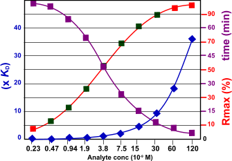
The figure shows the relation between the Rmax and the time to reach equilibrium. The red marks in the Rmax line indicate that the analyte concentration is either too low or too high.
| Concentration | Situation | |
|---|---|---|
| affinity | 0.1 - 10 x KD | |
| kinetics | 0.1 - 10 x KD | kd > 10-2s-1 |
| 1000 x KD | kd > 10-4s-1 |
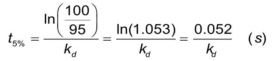
Dissociation time
For a reliable estimation of the dissociation rate, at least 5% of the analyte should be dissociated. For a dissociation rate of 1. 10-3 s-1 it will take about 1 minute to dissociate 5% of the bound ligand and at least 50 minutes to dissociate 95% of the bound analyte. The time to 5% dissociation can be estimated when the dissociation rate constant is known, with the next equation.
In situations with a slow dissociation, the 'short and long' injection scheme can minimize the experimental time significantly.
Regeneration
In order to reuse the sensor chip surface the analyte must be removed, but the ligand must stay intact. This so-called regeneration procedure has to be evaluated empirically because the combination of physical forces responsible for the binding are often unknown, and the regeneration conditions must not cause irreversible damage to the ligand (9), (10).
The most frequent regeneration method used, is to inject a low pH-buffer such as 10 mM Glycine pH 1.5–2.5 (10). This works probably because most proteins become partly unfolded and positively charged at low pH. The protein binding sites will repel each other and the unfolding will bring the molecules further apart (10).
Other procedures use high pH, high salt or specific chemicals to break the interaction. It is important to choose the mildest regeneration conditions that completely dissociate the complex. In addition, other molecules can be added such as antibodies, ligand and ligand analogues that bind to the analyte to diminish rebinding of the analyte during dissociation. More information can be found in de regeneration section.
References
| (1) | Myszka, D. G. et alKinetic analysis of a protein antigen-antibody interaction limited by mass transport on an optical biosensor. Biophysical Chemistry64: 127-137; (1997). |
| (2) | Myszka, D. G. et alExtending the range of rate constants available from BIACORE: interpreting mass transport-influenced binding data. Biophysical Journal75: 583-594; (1998). |
| (3) | Myszka, D. G.Improving biosensor analysis. J.Mol.Recognit.12: 279-284; (1999). |
| (4) | Rich, R. L. and Myszka, D. G.Survey of the year 2000 commercial optical biosensor literature. J.Mol.Recognit.14: 273-294; (2001). Goto reference |
| (5) | BIACORE ABKinetic and affinity analysis using BIA - Level 1. (1997). |
| (6) | BIACORE ABBia journal article. Bia Journal1: 5-7; (1999). |
| (7) | Rich, R. L. and Myszka, D. G.Survey of the year 2007 commercial optical biosensor literature. J.Mol.Recognit.21: 355-400; (2008). Goto reference |
| (8) | Cannon, M. J. et alComparative analyses of a small molecule/enzyme interaction by multiple users of Biacore technology. Analytical Biochemistry330: 98-113; (2004). |
| (9) | BIACORE ABBIACORE Getting Started. (1998). |
| (10) | Andersson, K. et alExploring buffer space for molecular interactions. J.Mol.Recognit.12: 310-315; (1999). Goto reference |