Curve fitting
After generating a sensorgram, the next step is fitting the curves. The first and only model to use is the 1:1 Langmuir interaction describing the single exponential of the data. With the first attempt, leave the bulk contribution and drift on zero and do not fit. Start by providing the initial fitting values and press “fit” to see the result. If the sensorgram consists of nice curves the fit will be ready in seconds; the fitted line follows the curves and will provide well defined values with small errors.
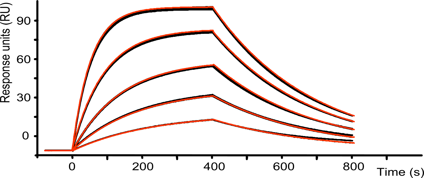
More realistic, optimization of the initial values and adjusting the fitting ranges may be necessary. This is normal and it is a good idea to fit the sensorgram with several initial values that differ a magnitude in scale. If, after fitting with different initial values, the results converge to the same values, it can be assumed that the values are well defined and robust. After the initial fittings, bulk contribution and/or drift can be fitted when necessary. Both bulk contribution and drift should be small compared to the curve response and proportional to the analyte concentration.
The next step is to critically compare the fitting with the measured curves. Does the fitting follow the curves? Are the calculated buffer jump values in line with the curves? Are the values of the parameters (Rmax, ka, kd) possible? Some instruments provide a quality control on the fitted parameters, however, always inspect the parameter values and the curves yourself.
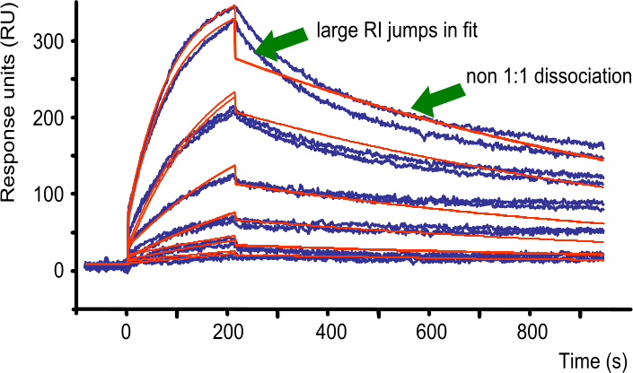
In the figure ‘1:1 fit with large RI jumps‘, the fit is not following the curves during the dissociation phase. By adding a larger buffer jump the program attempts to make the fit better. One other thing immediately apparent is that the overall response is too high. A way to solve this is to immobilize less ligand and repeat the experiment.
Other small problems, like small buffer jumps or low baseline drift can be solved with subtracting reference channels and blank (buffer only) injections (double referencing).
To validate further the interaction, several more steps are necessary. For instance, reverse the ligand and analyte and perform the experiments again. If you used the kinetic protocol, try an equilibrium experiment. Repeat the experiment with different batches of the same reagents to identify batch-to-batch variation. In all cases, a same value for kinetic constants is expected.
Read more
Read more about data fitting at the Data fitting introduction page.