Presenting a sensorgram
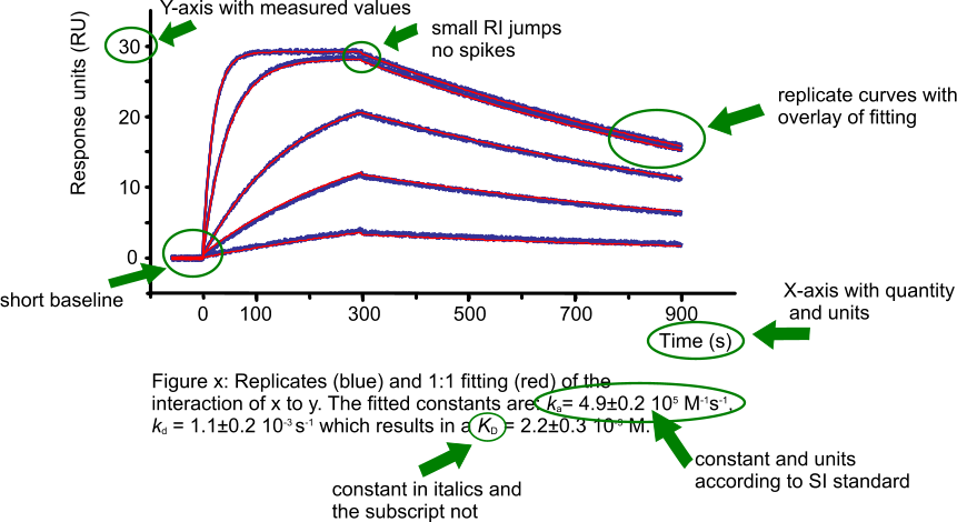
Presenting your fine results is the next step. To convince the public, you show them a nice sensorgram with a fit to the data (1). In the figure ‘High quality figure’ all the important parts of the sensorgram and legend are specified. In a publication, you probably give the kinetic values in the text or in a table. Please remember to use the SI standards for writing constants and units.
Looking at published results
When reading a publication, it has often one or two figures and a table with results. Now you have learnt to look at sensorgrams, you are not to be fooled any more by a representative curve and a table with values (2). The best way to check if the values are true is to simulate a curve with the kinetic constants from the table. Start with copying the representative curve to a drawing program. Simulate the curve in your kinetic evaluation software and copy the curve to the drawing program. Try to overlay the curve.
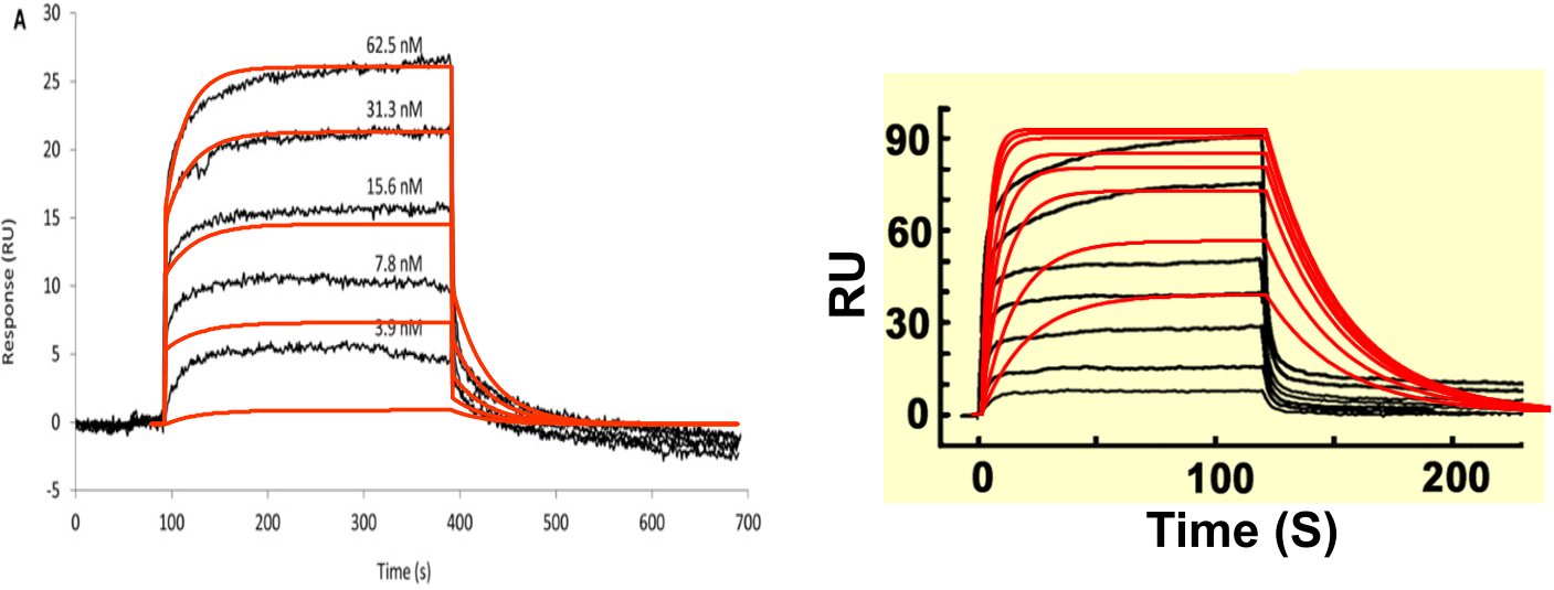
The figure ‘Simulated curves’ shows simulated curves over measured data from publications. Clearly, the simulations differ from the curves, which mean that the reported values are not representing the actual kinetics. Therefore, always show your curve with fittings and mention the values in a table. Most journals have the possibility to add additional information in the online supplemental section. Therefore there is no excuse for not showing your curves and fittings. .
Describing a Biosensor experiment
Equal important to the results is the way you have performed the experiments. You already know that it is very hard to repeat a published experiment. This is mainly because the author did not describe all the experimental conditions. This shortcoming is recognised and David Myszka proposed the TBMRFAADOBE (The Bare Minimum Requirements For An Article Describing Optical Biosensor Experiments) (2).
- instrument used in analysis
- identity, source, molecular weight of ligand and analyte
- surface type
- immobilization condition
- ligand density
- experimental buffers
- experimental temperatures
- analyte concentrations
- regeneration condition
- figure of binding responses with fit
- overlay of replicate analyses
- model used to fit the data
- binding constants with standard errors
Example text
As an example, here is a possible text for the methods part of a publication
The surface plasmon resonance experiments were performed using a BIACORE 2000 (GE Healtcare) equipped with a research-grade CM5 sensor chip. The ligand (60 kDa,>90% pure based on SDS–PAGE) was immobilized using amine-coupling chemistry. The surfaces of all four flow cells were activated for 7 min with a 1:1 mixture of 0.1 M NHS (N-hydroxysuccinimide) and 0.1 M EDC (3-(N,N-dimethylamino) propyl-N-ethylcarbodiimide) at a flow rate of 5 μl/min. The ligand at a concentration of 5 μg/ml in 10 mM sodium acetate, pH 5.0, was immobilized at a density of 200 RU on flow cell 2; flow cell 1 was left blank to serve as a reference surface. All the surfaces were blocked with a 7 min injection of 1 M ethanolamine, pH 8.0. To collect kinetic binding data, the analyte (34 kDa, >95% pure based on SDS–PAGE) in 10 mM HEPES, 150 mM NaCl, 0.005% P20, pH 7.4, was injected over the two flow cells at concentrations of 90, 30, 10, 3.3 and 1.1 nM at a flow rate of 60 μl/min and at a temperature of 20°C. The complex was allowed to associate and dissociate for 90 and 300 s, respectively. The surfaces were regenerated with a 5 s injection of 10 mM H3PO4. Triplicate injections (in random order) of each sample and a buffer blank were flowed over the two surfaces. Data were collected at a rate of 1 Hz. The data were fit to a simple 1:1 interaction model using the global data analysis option available within BiaEvaluation 3.1 software.
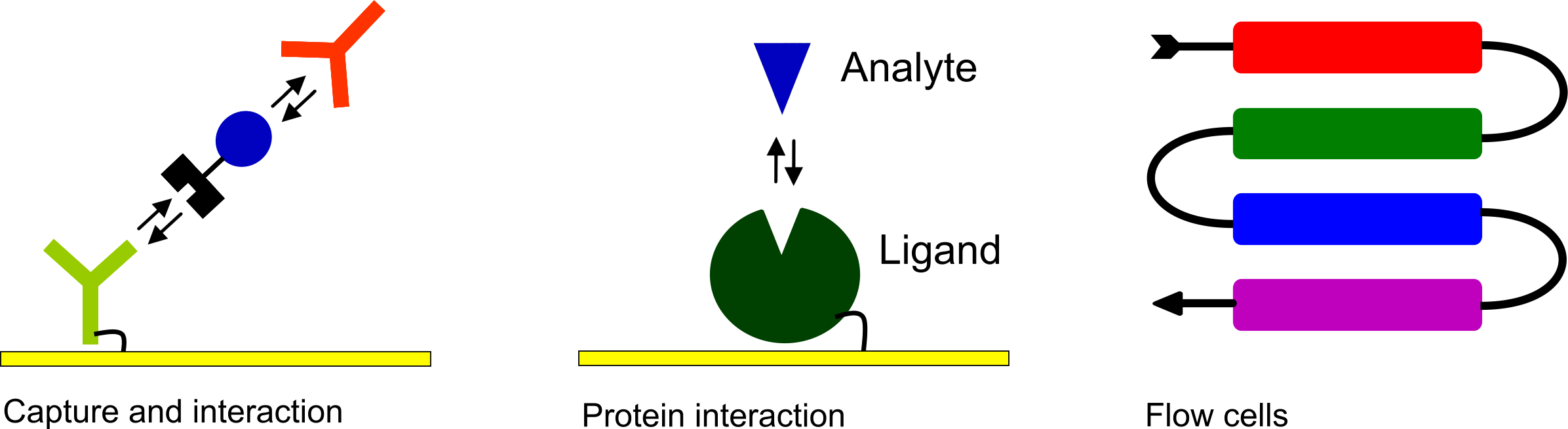
Cartoons
As an additional service to your readers, a figure depicting the layout of the interaction can be incorporated.
References
| (1) | Rich, R. L. and D. G. Myszka - Survey of the year 2007 commercial optical biosensor literature. J.Mol.Recognit. 21: 355-400; (2008). Goto reference |
| (2) | Rich, R. L. and D. G. Myszka - Grading the commercial optical biosensor literature-Class of 2008: 'The Mighty Binders'. J.Mol.Recognit. 23: 1-64; (2010). Goto reference |
| (3) | Yau, K. Y., M. A. Groves, S. Li, et al. - Selection of hapten-specific single-domain antibodies from a non-immunized llama ribosome display library. Journal of Immunological Methods 281: 161-175; (2003). |
| (4) | Wikipedia - International System of Units (https://en.wikipedia.org/wiki/International_System_of_Units). (2022). Goto reference |