Kinetic titration
The kinetic titration (single cycle kinetics) is useful with interactions which are difficult to regenerate or when regeneration is detrimental to the ligand (1). In addition, it can be used to determine the concentration and kinetic range of an interaction. During the kinetic titration, the analyte is injected from a low to high concentration with short dissociation times in between and a long dissociation time at the end. The short and long dissociation times will speed up the injection sequence. All the analyte injections are analysed in the same sensorgram with a special equation for kinetic titration. The model is based on the one to one binding interaction and is limited to five analyte injections (2). A mass transfer component (kt) and drift are added in de model.
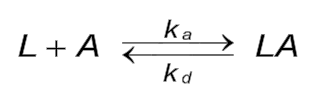
Reaction equation
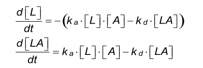
Differential equation
| Parameters | |
|---|---|
| L | concentration of free ligand in RU |
| A | concentration of free analyte in M |
| LA | concentration of ligand-analyte complex in RU |
| ka | association rate constant in M-1s-1 |
| kd | dissociation rate constant in s-1 |
Response calculation
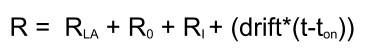
Because it is not possible to solve this type of injection with a differential model, a numeric model is used. In the numerical model each analyte injection is individually fit, and the total response calculated. The numerical model also contains terms for mass transport, drift and bulk refractive index mismatches.
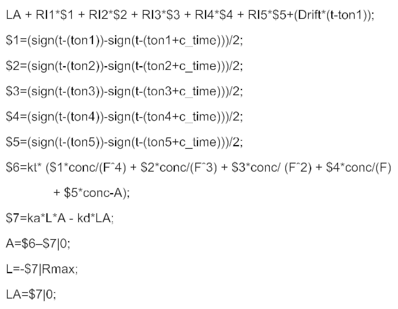
Numeric model
| Parameters | |
|---|---|
| LA | concentration of ligand-analyte complex in RU |
| RI | refractive index in RU |
| $x | injection time x |
| kt | mass transport coefficient |
| F | Dilution factor |
| Conc | concentration of free analyte in M |
| ka | association rate constant in M-1s-1 |
| kd | dissociation rate constant in s-1 |
| A | Analyte concentration in RU |
| L | Ligand concentration in RU |
| Name | Fit | Allow Neg. | Keyword | Initial value | Units |
|---|---|---|---|---|---|
| ka | global | No | No | 1e5 | M-1 s-1 |
| kd | global | No | No | 1e-3 | s-1 |
| Rmax | local | No | No | YMax | RU |
| kt | global | No | No | 2e7 | RU M-1 s-1 |
| RI1 | local | Yes | No | 0 | RU |
| RI2 | local | Yes | No | 0 | RU |
| RI3 | local | Yes | No | 0 | RU |
| RI4 | local | Yes | No | 0 | RU |
| RI5 | local | Yes | No | 0 | RU |
| Conc | No | No | Yes | M | |
| ton1 | No | No | Yes | s | |
| ton2 | No | No | Yes | s | |
| ton3 | No | No | Yes | s | |
| ton4 | No | No | Yes | s | |
| ton5 | No | No | Yes | s | |
| c-time | No | No | Yes | s | |
| F | No | No | Yes | ||
| Drift | Local | Yes | No | 0 | RU s-1 |
Although in the parameter table the RI and Drift are locally fit, they are in the model set to a constant of zero. It is better to start to fit the curves without these parameters. When the kinetic parameters are known, then it is possible to add refractive index bulk effect or drift.
| Name | Value | Units |
|---|---|---|
| ka | ka | M-1s-1 |
| kd | kd | s-1 |
| KD | kd/ka | M |
| Rmax | Rmax | RU |
| kt | kt | RU M-1s-1 |
| RI1 | RI1 | RU |
| RI2 | RI2 | RU |
| RI3 | RI3 | RU |
| RI4 | RI4 | RU |
| RI5 | RI5 | RU |
| Drift | Drift | RU s-1 |
Below an example of a sensorgram generated with the differential equations from above.
| Concentration (nM) | ka (M-1s-1) | kd (s-1) | RMax (RU) | ||
|---|---|---|---|---|---|
| local | global | global | global | ||
| - | 6.94 105 | 4 10-4 | 36 | ||
| 2 | |||||
| 4 | |||||
| 8 | |||||
| 16 | |||||
| 32 | |||||
References
| (1) | Dougan, D. A. et al - Effects of substitutions in the binding surface of an antibody on antigen affinity. Protein Eng 11: 65-74; (1998). Goto reference |
| (2) | Karlsson, R. et al - Analyzing a kinetic titration series using affinity biosensors. Analytical Biochemistry 349: 136-147; (2006). |