Kinetic models
There are a number of kinetic models that can be applied to the measured data. In general, one should use the simplest model to obtain kinetic values. However, not all data give the expected pseudo first-order reaction constants. Surface effects, such as immobilization heterogeneity or cross-linking and mass transfer or rebinding of analyte to the surface, can affect the data (1),(2), (3),(4).
Before fitting several models in search of the best-fit to the data, it is better to optimize the experimental conditions (5). In general, this results in additional experiments with different sensor chip types, immobilization chemistries, ligand densities, buffer compositions and flow rates. In addition, it is helpful to check the ligand and analyte for purity and integrity, directly before or after an SPR experiment.
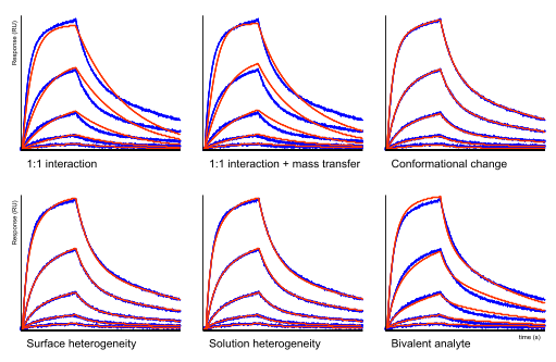
Below this text, there are six sensorgrams with a fitting through the measured data. It is clear that neither the 1:1 model nor the 1:1 model with mass transfer fits the data well. In these situations, often the conformational change model is applied (6),(7),(8). However, the heterogeneity models fit the data almost equally well as the bivalent analyte model. This example highlights the fact that model shopping is not the proper way to fit the data.
Start with a global fitting of the dissociation rate constant (kd). Use the obtained kd in the next global fitting with ka and Rmax (fix kd as a constant). Set the Bulk RI to zero and omit mass transfer and drift. After the fit is made, look at the fitted curves. Are they following the measured data? Is the dissociation fitted correctly? Are the association and Rmax calculated within the expected range?
From the initial fitting, decide which parameter (RI, mass transfer, drift) will make the fit better. The contribution of these parameters must be minimal. If this is not the case, the data is not 1:1 and new, better optimized sensorgrams should be made (5). Surface effects such as immobilization heterogeneity or cross-linking and mass transfer or rebinding of analyte to the surface can affect the data (1),(2),(3),(4).
Don’t go model shopping until you have a decent fit (6). Instead, before using other fitting models than the 1:1 Langmuir model make sure that:
- the system is clean and equilibrated
- the ligand is pure and homogenous
- the amount of ligand is low to minimize mass transport
- the analyte is pure and homogenous
- the analyte concentration range is wide enough (zero to saturation)
- the analyte buffer is matching the flow buffer minimizing bulk shift
- the injection time is long enough to give the association curvature
- the dissociation is long enough to give a reasonable signal decay
- blank injections are used for double referencing
- replicate analyte injections are done to prove the system stability
Global an local parameters
A robust fitting starts with high quality-data from several independent runs or experiments. In addition, the data must be cleaned of unwanted curves, regeneration parts and air-spikes. Further, reference subtraction and double referencing can be used to compensate for unmatched refractive indexes and baseline drift. The removal of injection and pump spikes will lower the Chi2 (9).
Many fitting programs allow you to calculate values for single curves or to calculate a single value for all the fitted curves. The first method is sometimes referred to as ‘local fitting’; the latter is called a ‘global analysis’ and will give the most robust answer. However, depending on the experimental set-up, some parameters should be fitted locally or globally.
ka
The association rate constant (ka) is determined by the properties of the ligand and analyte, temperature and buffer conditions. When during the experiment these conditions remain constant, the ka should be fit globally.
kd
The dissociation rate constant (kd) is determined by the properties of the ligand and analyte, temperature and buffer conditions. When during the experiment these conditions remain constant, the kd should be fit globally.
kobs
The fitted ‘observed rate constant’ (kobs) is fitted locally because it contains a term for the analyte concentration.
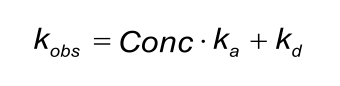
By constructing a plot of kobs versus the analyte concentration, the ka and kd can be determined. However, in many models the kobs is calculated from the concentration, ka and kd. In these cases, it makes no sense to draw a plot of kobs and analyte concentration since it will always be a straight line.
Mass transfer constants
Depending on the model, mass transfer constants are used to model the initial phase of the interaction where mass transfer may be prominent. Despite the differences, all mass transfer constants are globally fitted.
Rmax
Rmax is the maximal feasible signal between a ligand - analyte pair. Rmax is determined by the number of binding sites (Rligand * Vligand) and the size of the ligand and analyte molecules. Rmax is proportional to the relation between the molecular masses of the analyte and the ligand.

When one analyte species is injected – in different concentrations – over the same ligand surface, the theoretically the Rmax is the same for every injection. However, in practise this is not always the case, because binding sites may be lost due to regeneration conditions or incomplete regeneration.
The Rmax is always globally fitted for a single ligand analyte pair.
Because Rmax is determined by the size of the ligand and analyte, Rmax is fitted locally when different analyte molecules are used over the same surface.
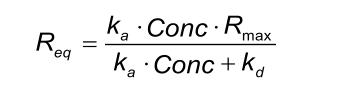
Req
Req is the signal when the binding between ligand and analyte is at equilibrium. To reach this state, the injection period should be such that association and dissociation are at steady state. Req is determined by the maximal number of binding sites (Rmax), kinetics (ka, kd) and the concentration of the analyte molecule (Conc.).
When an analyte is injected in different concentrations over a ligand surface, then the Req equals the number of occupied binding sites.
Because Req depends on Rmax, ka and kd, these parameters must be globally fitted before the local Req can provide information about the number of occupied binding sites.
RI
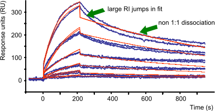
The bulk signal (RI) is caused by refractive index differences between the flow buffer and the buffer with the analyte (protein concentration, dilution and other buffer components). The RI is often used to allow the curve to fit better. If RI jumps in the measured curves are large, more care should be used to eliminate bulk effects by matching the buffers. When the RI jumps in the fit are large compared to the curve jumps, it means that the model does not fit the data well (7). More should be done to eliminate non 1:1 curve behaviour by optimizing experimental conditions.
The RI is proportional to the analyte concentration and should be small compared to the overall response. Therefore, RI is always fitted locally. RI is only applicable to the association phase.
Drift
Drift comes mostly from non-optimally equilibrated surfaces. Referencing and double referencing can compensate for the drift but some residual drift will sometimes remaining. Fit the curves first without a drift component. Then add a drift component in the final fitting with initial values from the previous result. The contribution of the drift should be low ( < ± 0.05 RU s-1). Drift is fitted locally.
Chi2
The Chi2 gives a measure of the accuracy of the fitting. This parameter is determined using all curves, which are simultaneously fitted. The Chi2 increases with the number of curves. The fitting process will give one Chi2.
Residuals
The residuals are graphical representations of the accuracy of the fitting. Although a fitting can give low Chi2, the residuals provide a better insight if a model is accurate or not. A good fit will have absolute residuals that are in the order of the machine noise. For every fitted curve, there is a set of residuals.
References
| (1) | Edwards, P. R., A. Gill, K. D. V. Pollard, et al. Kinetics of protein-protein interactions at the surface of an optical biosensor. Analytical Biochemistry 231: 210-217; (1995). |
| (2) | Glaser, R. W. Antigen-antibody binding and mass transport by convection and diffusion to a surface: a two-dimensional computer model of binding and dissociation kinetics. Analytical Biochemistry 213: 152-161; (1993). |
| (3) | Myszka, D. G., T. A. Morton, M. L. Doyle, et al. - Kinetic analysis of a protein antigen-antibody interaction limited by mass transport on an optical biosensor. Biophysical Chemistry 64: 127-137; (1997). |
| (4) | Schuck, P. - Kinetics of ligand binding to receptor immobilized in a polymer matrix, as detected with an evanescent wave biosensor. I. A computer simulation of the influence of mass transport. Biophysical Journal 70: 1230-1249; (1996). |
| (5) | Rich, R. L. and D. G. Myszka - Survey of the year 2006 commercial optical biosensor literature. J.Mol.Recognit. 20: 300-366; (2007). Goto reference |
| (6) | Rich, R. L. and D. G. Myszka - The Revolution of Real-Time, Label-Free Biosensor Applications. (2011). Goto reference |
| (7) | Rich, R. L. and D. G. Myszka - Grading the commercial optical biosensor literature-Class of 2008: 'The Mighty Binders'. J.Mol.Recognit. 23: 1-64; (2010). Goto reference |
| (8) | Rich, R. L. and D. G. Myszka - Extracting kinetic rate constants from binding responses. (2009). Goto reference |
| (9) | Katsamba, P. S., I. Navratilova, M. Calderon-Cacia, et al. - Kinetic analysis of a high-affinity antibody/antigen interaction performed by multiple Biacore users. Analytical Biochemistry 352: 208-221; (2006). |