Validation
Validation of the fitting results is an essential step. Do not believe the calculated values without checking! Always inspect the curves and residuals. In addition, inspect the calculated values (Rmax, RI, Req, ka, kd). Do they make sense?
Curve inspection
The best way to see if a fitting follows the measured data is by visual inspection (1), (2). Deviations of the fitting from the actual data are easily found by inspection of the residuals. Discrepancies between the fitted model and the experimental data are of two kinds (3):
Random deviations
The random deviations should reflect normal scatter in the experimental data. This kind of deviation should have a normal distribution meaning that high and low deviations are occurring at the same amount.
Systematic deviations
The systematic deviations arise because the model is an inadequate description of the experimental situation. The association or dissociation is faster or slower or the calculated RI jump is smaller. By careful inspection of the deviation, you can get clues about what is the cause of the deviation.
Examine the Chi2-values and the residual plots for the fitting. Points in the residual plot are scattered within a band. The width of the band at a given time indicates the noise level, while the shape of the band reveals systematic differences between the fitted curve and the experimental data (4), (5). For typical sensorgrams, the noise level should not exceed the normal noise level of the instrument. In the global analyses, the noise level may be somewhat higher.
Checking the results
Start by inspecting the kd. In order to have a valid calculation the dissociation should be at least 5% of the starting value. If the value is lower than 1.10-5 s-1 the dissociation time should be at least 90 minutes (see table). The ka should be in the valid range of the instrument. In addition, are the calculated variables biologically relevant?
The Rmax is also calculated during the fit. The Rmax reflects the maximal response when all ligand is occupied. This will be hardly the case, even if you inject a 100 times the KD. In addition, the time needed to reach Rmax (at Req) can be beyond the injection time of the instrument. Use the Rmax and Req to judge if the curves following a 1:1 kinetic. If the fitted Rmax is very high compared to the response of the curves this can be an indication that the fit is wrong.
How is the standard error (SE)? (6). The standard error of the calculated values is often very low, indicating that the value is well defined. Do not use the standard error in the reporting of your values. If you want to report an error to your values, you have to repeat the experiment and calculate the standard deviation (check Wikipedia).
| Instrument | ka (M-1s-1) | kd (s-1) | KD (M) |
|---|---|---|---|
| Biacore 2000 | 103 – 5.106 | 5.10-6 – 10-1 | 10-4 – 2.10-10 |
| Biacore 3000 | 103 – 107 | 5.10-6 – 10-1 | 10-4 – 2.10-10 |
| Biacore X100 | 103 – 107 | 1.10-5 – 10-1 | 10-4 – 1.10-10 |
| SensiQ Pioneer | < 108 | 1.10-6 – 10-1 | 10-3 – 10-12 |
| IBIS-MX96 | 10-5 – 10-12 | ||
| Plexera HT analyzer | 102 – 106 | 10-2 – 10-5 | 10-6 – 10-9 |
| Reichert SR7500DC | 10-3 – 10-9 | ||
| SierraSensors SPR-2 | 103 – 106 | 10-1 – 10-5 | 10-4 – 10-11 |
Chi2
The Chi2 shows also information about the goodness of fit but is less affected by the large number of data points. However, the Chi2 is difficult to interpret (8). First, it depends strongly on the average signal level and therefore a generally acceptable Chi2 cut-off cannot be established. Second, it is not well adapted for time series data, because there is typically a strong correlation between data points in close temporal proximity. However, the Chi2 can be used as a global measure for the residual noise. For a good fitting, the square root of Chi2 is of the same magnitude as the noise of the measurement.
Validating the model
In the cases that the fitting is not optimal, you can use another model. However, this model surfing will not give you any better understanding of what is happing during the interaction. Instead of applying various models to measured curves, try to design proper experiments. So:
- Use different immobilization densities and sensor chips. Two or more ligand densities can unmask ligand heterogeneity and mass transfer effects. Different sensor chip types can give insight in possible matrix effects.
- Vary buffers. Different buffers can give different effects on binding or matrix.
- Use an in-line reference surface and blank injection for subtraction of bulk effects and checking the specificity. The reference surface should be designed to mimic the specific surface, as close as possible but without the ligand of interest.
- Vary flow rates. Different flow rates can identify mass transfer. High flow rates will reduce the diffusion distance, speed up sample transition and improve reference subtraction. Use flow rates of at least 30 µ/min or higher and use the best injection command for minimum sensorgram distortion.
- Use the correct analyte concentrations. For affinity determination, use a concentration of 0.1 – 10 KD of analyte. For kinetic analysis use 0.1 - 10 KD when KD > 10-2 s-1 or 1000 KD when KD < 10-4 s-1.
- Use various analyte concentrations and inject at random. In this way, cumulative effects related to analyte concentration are avoided. In addition, possible carryover effects can be detected.
- Repeat the experiment with a new prepared ligand surface and a different batch of the analyte. Average the values.
- Vary analyte contact times. Use various contact times at high analyte concentrations (100% Rmax) to discriminate between dependent and independent binding reactions.
- Switch the role of ligand and analyte. In theory, the kinetics should not change for a normal 1:1 reaction when ligand and analyte are switched.
- Try equilibrium experiments. At equilibrium (steady state), the KD can be calculated and later be compared with kinetic experiments. They should be comparable.
- Use Global analysis. Global analysis gives more robust and reliable fittings. Use five or more concentrations over the range of 0.1 – 10 KD in one fitting for the best results. The residuals should not exceed 1/10 of the response.
- Use fraction collection. Fraction collection and reinjection can identify two forms of analyte (see independent versus linked reactions).
- Vary temperature. Varying temperature can give valuable insight in the binding kinetics and type of binding. Do not forget to normalize/calibrate after a temperature change.
- Adjust data collection rate. Some fast on and off rates can be detected by adjusting to a faster data collection rate.
- Check self-consistency of the calculated values (see below).
- Use a simulation program. Simulation software allows visualization of clean curves with the calculated parameters. The simulated curves should be similar to the measured curves.
Self-consistency of the data
Examine the results for consistency over a range of analyte concentrations. In the global analysis method, this is performed in the fitting procedure. Nevertheless, inspect each of the fitted curves for deviations. When fitting one curve at the time, check if the constants vary with the analyte concentration. If so, the model is probably inadequate.
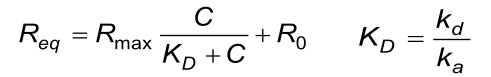
Some simple test can be done to check if the reported values are consistent (7). The calculated KD value obtained from the equilibrium reaction must be the same as the KD calculated from de individual ka and kd values from the association phase.
The calculated (fitted) kd from the association phase must approximately be the same as from the dissociation phase.
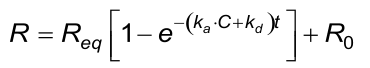

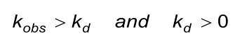
The calculated (fitted) observed rate constant (kobs) in the association phase must comply with the next two conditions. Beware that the evaluation software the kobs calculates from ka, C and kd.

Further reading
The next list contains references that are very interesting to read. So I suggest you look them up and study.
| 1. | Cornish-Bowden, A. - Detection of errors of interpretation in experiments in enzyme kinetics; Methods ;24: 181-190; (2001). |
| 2. | kalinin, N. L. et all - Effects of solute multivalence on the evaluation of binding constants by biosensor technology: studies with concanavalin A and interleukin-6 as partitioning proteins; Analytical Biochemistry ;228: 238-244; (1-7-1995). |
| 3. | Roden, L. D. and Myszka, D. G. - Global analysis of a macromolecular interaction measured on BIAcore; Biochem.Biophys.Res.Commun. ;225: 1073-1077; (23-8-1996). |
| 4. | Wu, Z. et all - Ligand binding analysis of soluble interleukin-2 receptor complexes by surface plasmon resonance; J.Biol.Chem. ;270: 16045-16051; (7-7-1995) |
References
| (1) | Morton, T. A. et al - Interpreting complex binding kinetics from optical biosensors: a comparison of analysis by linearization, the integrated rate equation, and numerical integration. Analytical Biochemistry227: 176-185; (1995). |
| (2) | Cornish-Bowden, A. - Detection of errors of interpretation in experiments in enzyme kinetics. Methods24: 181-190; (2001). Goto reference |
| (3) | BIACORE AB - BiaEvaluation 2.0. (1998). |
| (4) | De Crescenzo, G. et al - Real-Time Kinetic Studies on the Interaction of Transforming Growth Factor alpha with the Epidermal Growth Factor Receptor Extracellular Domain Reveal a Conformational Change Model. Biochemistry39: 9466-9476; (2000). |
| (5) | Onell, A. and Andersson, K. - Kinetic determinations of molecular interactions using Biacore - minimum data requirements for efficient experimemtal design. J.Mol.Recognit.18: 307-317; (2005). |
| (6) | BIACORE AB - Kinetic and affinity analysis using BIA - Level 1. (1997). |
| (7) | Schuck, P. and Minton, A. P. - Kinetic analysis of biosensor data: elementary test of self-consistency. Trends Biochem.Sci.21: 458-460; (1996). |
| (8) | Onell, A. and Andersson, K. - Kinetic determinations of molecular interactions using Biacore - minimum data requirements for efficient experimemtal design. J.Mol.Recognit.J.Mol.Recognit. (18): 307-317; 2005. |