Data fitting
Theory
The goal of data fitting is to draw a line through a data set. Before fitting the data, we need a model. A model is a formal mathematical representation of a chemical or physiological idea. To be useful, the model must be expressed as an equation that defines Y, the outcome of a measurement, as a function of X and one or more variables to be fitted. The term variable is used to refer to the terms in the equation to be fitted. With non-linear regression, the term variable does not refer to X and Y (1).
For instance, the law of mass action is the model for the simplest binding reaction between two proteins (1),(2). The reaction between immobilized ligand (L) and an analyte (A) can be assumed to follow a pseudo first order kinetics (3),(4),(5). The reaction equation looks like this:

During the association phase the complex [LA] increases as a function of time. The differential rate equation describes the relation between the parameters:
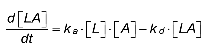
In the equation for complex formation the ka is the association rate constant which describes the rate of complex formation, i.e. the number of LA complexes formed per second in a one molar solution of L and A. The units of ka are M-1s-1 and are typically between 1.103 and 1.107 in biological systems.
kd is the dissociation rate constant which describes the stability of the complex, i.e. the fraction of complexes that decays per second. The unit of kd is s-1 and is typically between 1.10-1 and 1.10-6 in biological systems. A kd of 1.10-2 s-1 = 0.01 s-1. This means that 1 percent of the complexes decay per second.
Integration
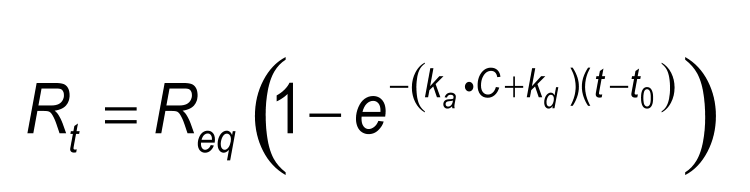
Although the differential rate equation describes the one to one Langmuir reaction accurately, it is not useful as a model to fit to a curve. By integrating the differential rate equation, sensorgrams can be analysed directly using non-linear methods (6). This is because integrated rate equations describe the whole curve as opposed to the differential rate equations, which describe the slope of a curve.
The classical Langmuir surface adsorption (7) can be described with the following integrated rate equation(6)
Numerical integration
While simple rate equations are easily integrated, the more complex (e.g. with mass transport parameters) are not. The more complex rate equations are resolved by numeric calculations. Using numerical integration (a.k.a. non-linear regression) has also the advantage that global analysis can be linked in. This means that several curves are fitted simultaneously giving a single and more robust answer for the rate constants (8).
Non-linear regression
Non-linear regression is a more general approach to data fitting because all models that define Y as a function of X can be fitted. The process will find the values for the variables giving the closest fit, reducing the sum-of-squares (SS) to a minimum. The SS is calculated from the vertical distances between the curve and the measured points.

Non-linear regression can fit complex models by an iterative process, which starts with initial values provided by the user. The iterative process goes on until the convergence criteria are matched. For instance, when two iterations change the SS by less than 0.01%.
The initial values are estimates of the real values. During the iterative process, the program adjusts these values to improve the fit. Initial values matter more when the data has a lot of scatter or does not span the whole curve. Depending on the initial values, different results may follow. This phenomenon is the result of the search for a local minimum.
In the figure 'Local minimum', there is a sinus curve. Searching for the true minimum can start on either side of the curve. Only one side will give the true minimum. So, when a fitting does not work, try different initial values in steps of 100 times difference.
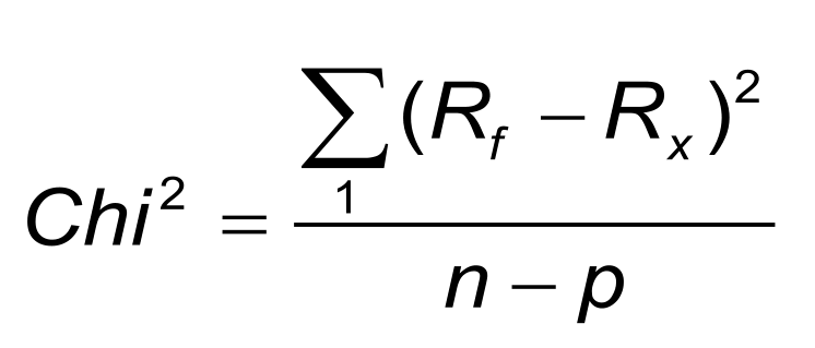
Often the Chi2-value is given after the fitting is done. The Chi2-value shows information about the goodness of fit. For a good fitting, the Chi2 is in the same magnitude as the noise of the used system (but check the validation section).
Assumptions with non-linear regression
The results of non-linear regression are meaningful only if the following assumptions are true (or nearly true):
- The model is correct. Non-linear regression adjusts the variables in the chosen equation to minimize the sum-of squares. It does not attempt to find a better equation.
- The variability of values around the curve follows a Gaussian distribution. Although no biological variable follows a Gaussian distribution exactly, it is sufficient that the variation is approximately Gaussian.
- The SD of the variability is the same everywhere, regardless of the value of X. If the SD is not constant but rather is proportional to the value of Y, the data should be weighted to minimize the sum-of-squares of the relative distances.
- The model assumes that X is known exactly. This is rarely the case, but it is sufficient to assume that any imprecision in measuring X is very small compared to the variability in Y.
- The errors are independent. The deviation of each value from the curve should be random, and should not be correlated with the deviation of the previous or next point.
References
| (1) | Graphpad Software - Graphpad Prism. (2022). Goto reference |
| (2) | Elwing, H. - Protein absorption and ellipsometry in biomaterial research. Biomaterials 19: 397-406; (1998). |
| (3) | Bjorquist, P. and Bostrom, S. - Determination of the kinetic constants of tissue factor/factor VII/factor VIIA and antithrombin/heparin using surface plasmon resonance. Thrombosis Research 85: 225-236; (1997). |
| (4) | O'Shannessy, D. J. et al - Determination of rate and equilibrium binding constants for macromolecular interactions using surface plasmon resonance: use of nonlinear least squares analysis methods. Analytical Biochemistry 212: 457-468; (1993). |
| (5) | Johnsson, B. et al - Immobilization of proteins to a carboxymethyldextran-modified gold surface for biospecific interaction analysis in surface plasmon resonance sensors. Analytical Biochemistry 198: 268-277; (1991). |
| (6) | BIACORE AB - BIACORE Technology Handbook. (1998). |
| (7) | BIACORE AB - Bia Journal Article. Bia Journal 2: 18(1998). |
| (8) | Karlsson, R. and Falt, A. - Experimental design for kinetic analysis of protein-protein interactions with surface plasmon resonance biosensors. Journal of Immunological Methods 200: 121-133; (1997). Goto reference |