Equilibrium analysis
For equilibrium analysis (a.k.a. steady state analysis), the injection of analyte must be long enough to reach steady state. Only when steady state is reached, it is possible to determine the equilibrium dissociation constant KD from a plot of the response at equilibrium versus the analyte concentration (1).
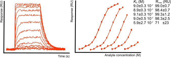
For equilibrium analysis, it is not necessary to saturate the ligand as long as the equilibrium curve has enough curvature to be fit properly. In the equilibrium fitting example figure, subsequent points are left out in the analysis. For a reliable result, roughly 40 to 50 % of the ligand must the saturated.
An important experimental consideration is the time taken to reach equilibrium (see the sensorgram tutorial). Low concentrations of analyte will take longer to reach equilibrium. If the time needed is longer than feasible with the injection pump, it is possible to add the analyte to the flow buffer (2). The analyte concentration is raised in steps and after the highest concentration is done, the process is reversed with different lower concentrations to show that the system is reversible. An advantage is that the procedure is without any regeneration step.