The exponential

The first result from a SPR experiment is the sensorgram. Each sensorgram contains a world of information for the trained eye. Therefore, it is essential to recognize good from bad curves. A bad curve represents a bad experiment, producing bad results from which conclusions cannot be made. And be sure, there is a lot of rubbish in the SPR literature! For example, please read the articles from D.G. Myszka and R.L. Rich (1),(2).

A good understanding of the binding curves is the first step in interpreting the data. Let us start with the binding between two dissimilar molecules. One molecule, the analyte (A), binds to one molecule, the ligand (L) in a reversible way. The velocity or rate of binding (association) is denoted by the association rate constant k_a in M^-1s^-1. The breaking up of the complex (dissociation) is denoted by the dissociation rate constant k_d in s^-1. The quotient of the k_d/k_a defines the equilibrium dissociation constant K_D in Molar which provides the analyte concentration that will saturate 50% of the ligand. Equation 1 shows the rate equation for a 1 to 1 interaction between the ligand and analyte.

At the start of the interaction, all the ligand is unbound and the baseline is measured. By introducing the analyte, ligand-analyte (LA) complexes are formed. The amount (concentration) of complex formed by the interaction can be calculated with the differential equation 2.

Integrating equation 2, gives an integrated rate equation, which describes the complete interaction curve as opposed to the differential rate equation which describes the slope of the curve.

Equation 3 describes a simple exponential binding profile (see the exponential e). No other curve shapes such as parabolic, hyperbolic, concave and convex can describe the binding profile. Although the curve is a single exponential, the shape depends on several parameters. R_t is the response at time t and R_eq is the maximal response (equilibrium response) which can be reached with the injected analyte concentration; k_a is the association rate constant; k_d the dissociation rate constant and C the analyte concentration. The term (t-R₀) is the time interval of the interaction.

In the same way, equation 4 describes the exponential dissociation where R₀ is the response at the start of the dissociation and R_t the response at time t. From the formula it can be seen that the dissociation only depends on the dissociation rate constant k_d.

Curve examples

Now, train yourself to recognize an exponential binding curve. In the figure below, some sensorgrams are given as an overview of the possible curve shapes, which are all still exponential but differ in kinetics. The curves differ in association and dissociation rate, but the shape is always an exponential.

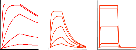
From left to right the curves have a relative fast association rate and relative slow dissociation rate, a moderate association and dissociation rate and a fast dissociation rate. However it is not possible to compare the association from the association phase alone since the association rate is also dependent on the analyte concentration; remember equation 2 above.

Look now at the following curves.

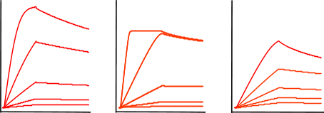
The figure 'Mass transfer limited curves' shows sensorgrams that have curves with an initial binding profile, which appears to be linear. This is an example of (partially) mass transport limited kinetics. Directly after the analyte injection starts, the binding of the analyte to the ligand is faster than the analyte diffusion towards the ligand, creating a shortage of analyte at the surface. Therefore, the interaction is diffusion limited instead of kinetic limited. It is easy to incorporate mass transport limitation in the fitting models but it is better to avoid this by proper design of the experiment. For instance by lowering the ligand density or increasing the flow rate.

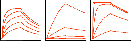
The next sensorgrams are often referred to as having biphasic binding responses. Biphasic responses are said to consist of a fast and slow interaction. And because a biphasic response can be described equally well by different models (1) it is virtually impossible to solve the interaction mechanism by modelling alone. In case of a biphasic curve, more optimisation of the experimental conditions is necessary. Don’t try to fit these curves!

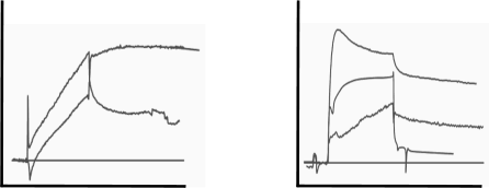
The next two sets of curves are seen in cases like buffer jumps, spikes and drift. Although drift can be added to the fitting model, it is better to avoid drift by proper equilibration of the system. After immobilisation, drift is often very strong. The easiest way to equilibrate is to run flow buffer overnight. When starting your measurements, incorporate several dummy injections (running buffer) to validate the stability of the system. Always try to match the flow and sample buffer to avoid buffer jumps at the beginning and the end of the injections. The spiky and wobbly sensorgrams are a warning to clean your system. Make new degassed reagents and start over designing your experiment.