How low can you go?
In SPR experiments, low responses are preferred over high responses. This is because high responses in general are affected by mass transport and non 1:1 interactions (6),(8). But how low can you go? This depends in the first place on the instrument you have chosen. The signal should be above the noise level of the baseline. The curves should be easily recognisable and replicates should overlay (4),(7).
To determine the noise level of the instrument, first equilibrate the system to minimize drift. Then inject flow buffer several times and observe the average response. The average response level is the starting point for the next experiments. In addition, check the shape of the curves. If there is drift or the curves are not level shortly after the start of the injection, equilibrate better or clean the instrument.
Then calculate the amount of ligand to immobilize to get a proper signal. This will be a matter of trial and error since you do not know the amount of active ligand, which is available after immobilization. As a starting point, calculate a response of 100 RU. After immobilization, it is essential to equilibrate the system since the immobilization uses several high-concentration solutions. The best method to check the equilibration is to inject flow buffer several times and then monitor the baseline.

When flow buffer equilibration is reached, inject analyte from a low to a high concentration. Take a broad range of concentrations, e.g. 0.1 nM – 1 µM. The fastest method is the kinetic titration method (3). Between the injections there is a short dissociation period and then a longer one after the last injection. These first injections give you an idea about the ligand activity, useful analyte concentration range, kinetics (association and dissociation rate) and the maximal response of the interaction. Knowing this, proper changes to the ligand immobilization level or analyte concentration range can be made. In addition, you can optimize the association and dissociation injection period.
When the dissociation is very slow, a regeneration solution (e.g. low pH, high salt) can be used to remove the analyte. However, regeneration can be problematic. It should remove the analyte completely but the ligand must remain intact on the surface. Therefore, use the mildest regeneration solution and shortest contact time possible. In addition, regeneration can cause matrix effects (drift) which can look like there is still analyte on the surface. Make sure the system is fully equilibrated after regeneration. Use the washing command and extend the equilibration time when necessary. This will be a matter of testing (1),(2).
Know your system:
- immobilization level: immobilize enough ligand to get proper signals above the noise level but keep the immobilization level low enough to avoid mass transport or steric hindrance.
- analyte concentration range: use an analyte concentration range between 0.1 – 10 times the expected KD.
- association and dissociation time: adjust the injection times so that the association is long enough to have curvature and the time during dissociation is long enough to have at least a 5% decrease in response.
- regeneration conditions: adjust the regeneration solution, contact time and post-wash routines to have the best regeneration without drift or shifts.
Let the data be your guide by reproducing the response of the interaction (5).
Example of the interaction of zinc with B2GPI and HPRG.
The surface plasmon resonance experiments were performed using a BIACORE 2000 (GE Healthcare) equipped with a research-grade CM5 sensor chip. The ligand (44 or 74 kDa, >90% pure based on SDS–PAGE) was immobilized using amine-coupling chemistry. The surfaces of the flow cells were activated for 7 min with a 1:1 mixture of 0.1 M NHS (N-hydroxysuccinimide) and 0.1 M EDC (3-(N,N-dimethylamino) propyl-N-ethylcarbodiimide) at a flow rate of 5 μl/min. The ligand at a concentration of 5 μg/ml in 10 mM sodium acetate, pH 5.0, was immobilized at a density of approximately 1200 - 1500 RU; flow cell 1 was left unmodified to serve as a reference surface. All the surfaces were blocked with a 7 min injection of 1 M ethanolamine, pH 8.0.
| Proteins used in the experimenR |
||||
|---|---|---|---|---|
| Channel | protein | Mr | Bound | Density |
| (Da) | (RU) | (pmol/mm2) | ||
| 1 red | unmodified | |||
| 2 green | B2GPI | 44000 | 1150 | 0.026 |
| 3 blue | HPRG | 74000 | 1525 | 0.021 |
| 4 purple | B2GPI open | 44000 | 1280 | 0.029 |
To collect kinetic binding data, zinc chloride in 10 mM HEPES, 150 mM NaCl, 0.005% P20, pH 7.4, was injected over the two flow cells at concentrations of 10, 5, 2.5, 1.25, 0.63, 0.31, 0.16, 0.08 µM at a flow rate of 30 μl/min and at a temperature of 25°C. The complex was allowed to associate and dissociate for 90 and 300 s, respectively. The surfaces were regenerated with a 5 s injection of 3 mM EDTA. Duplicate injections (in random order) of each sample and a buffer blank were flowed over the four surfaces. Data were collected at a rate of 1 Hz. The data were fit to a simple steady-state affinity model using the Scrubber software.
References
| (1) | BIACORE AB - BIACORE Getting Started. (1998). |
Example of Carboxy Anhydrase Isozyme II and acetazolamide
The surface plasmon resonance experiments were performed using a BIACORE 2000 (GE Healthcare) equipped with a research-grade CM5 sensor chip. The ligand (CA II, 29 KDa) was immobilized using amine-coupling chemistry. The surface of the flow cell 1 was activated for 7 min with a 1:1 mixture of 0.1 M NHS (N-hydroxysuccinimide) and 0.1 M EDC (3-(N,N-dimethylamino) propyl-N-ethylcarbodiimide) at a flow rate of 5 μl/min. The ligand at a concentration of 15 μg/ml in 10 mM sodium acetate, pH 5.0, was immobilized at a density of approximately 3500 RU. The surface was blocked with a 7 min injection of 1 M ethanolamine, pH 8.0. Flow cell 3 was left unmodified to serve as a reference surface.
To collect kinetic binding data, Acetazolamide in 10 mM HEPES, 150 mM NaCl, 0.005% P20, pH 7.4, was injected in the concentrations of 1000, 333, 37, 12.3, 4.11 and 1.37 nM at a flow rate of 100 μl/min and 25°C. The complex was allowed to associate and dissociate for 170 and 300 s, respectively. Regeneration was not necessary is this system. Triplicate injections (in random order) of each sample and buffer blanks were flowed over the four surfaces. Data were collected at a rate of 10 Hz. The data were fit to a simple 1:1 model using the global data analysis option available within Scrubber software.
How low did you go?
Tell us, how low did you go? Show us your sensorgrams and analysis.
Other examples
Creoptix sensors
![]() Example of Carboxy Anhydrase Isozyme II and Acetazolamide.
Example of Carboxy Anhydrase Isozyme II and Acetazolamide.
The kinetics experiments were performed using a Creoptix WAVE Delta (Creoptix AG) equipped with a research-grade 4PCH sensor chip. The ligand (CA II, 29 KDa) was immobilized using amine-coupling chemistry. The surface of all flow cells (1 to 4) was activated for 7 min with a 1:1 mixture of 0.1 M NHS (N-hydroxysuccinimide) and 0.1 M EDC (3-(N,N-dimethylamino) propyl-N-ethylcarbodiimide) at a flow rate of 10 μl/min. The ligand at a concentration of 5 μg/ml in 10 mM sodium acetate, pH 5.0, was immobilized at a density of approximately 860 pg/mm2 (1 pg/mm2 = 1 RU) in flow cell 3. The ligand at a concentration of 20 μg/ml in 10 mM sodium acetate, pH 5.0, was immobilized at a density of approximately 8100 pg/mm2 (1 pg/mm2 = 1 RU) in flow cell 2. The surfaces were blocked with a 7 min injection of 1 M ethanolamine, pH 8.0. Flow cell 1 was left unmodified to serve as a reference surface.
To collect kinetic binding data, Acetazolamide in PBS, 3% DMSO, pH 7.4, was injected in the concentrations of 1000, 333, 111, 37, 12.3, 4.11 and 1.37 nM at a flow rate of 100 μl/min and 25°C. The complex was allowed to associate and dissociate for 60 and 300 s, respectively. Regeneration was not necessary is this system. Triplicate injections (in different orders) of each sample and buffer blanks were flowed over the four surfaces in parallel. Data were collected at a rate of 10 Hz. The data with high Rmax were fit to a mass transport limited model (with bulk correction of 20% and 1% in association and dissociation, respectively), while the low Rmax data were fit to a simple 1:1 model (with bulk correction of 50% and 10% in association and dissociation, respectively). In both cases the data were fit using the global data analysis available within Creoptix WAVE control software.
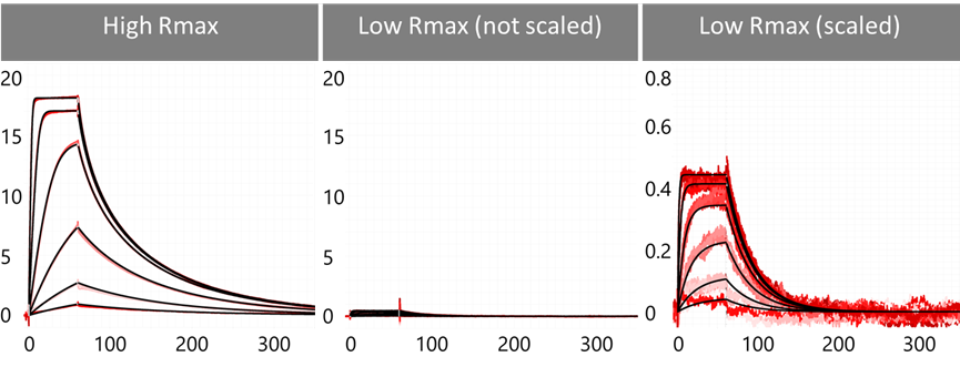
| High Rmax | Low Rmax | Units | |
|---|---|---|---|
| Rmax | 18.658 | 0.473 | pg/mm2 |
| ka | 1.31 10+6 | 7.45 10+5 | M-1s-1 |
| kd | 4.06 10-2 | 3.29 10-2 | s-1 |
| KD | 31.0 | 44.2 | nM |
| Kt | 6.01 10+6 | n.a. | s-1 |
| note: 1 pg/mm2 is equal to 1 RU | |||